Lessons from a decade of failed austerity

 “Worst of all is the orthodox theory that bad trade calls for economy – economy in all new development, both public and private, economy in bankers’ loans, economy in wages, economy in social services, economy in employment, economy in enterprise, ‘freedom from thought.’ This disastrous doctrine dominated British policy between the wars … The Labour Party was right when it declared that this was the exact reverse of the truth, and that the supposed cure only made the disease worse.” [1]

The Labour Party of 1944 castigated the notion of ‘economy’; policymakers in 2010 spoke of ‘consolidation’; most people talk about ‘austerity’. The Coalition government resurrected various soundbites: an economy ‘living beyond its means’; calling for ‘good housekeeping’ and ‘cutting one’s coat to fit one’s cloth’. They fell in line with a global appeal, with the OECD arguing in November 2009:

Credible medium-term consolidation programmes should be announced already now, in order to strengthen market expectations about the determination of governments to return to sustainable fiscal positions. (p. 63)[2]

The economic ideal was rebranded as ‘expansionary fiscal contraction’, infamously associated with the Harvard economist Alberto Alesina. Amounting only to the old wine of ‘crowding out’ in a new bottle, getting government out of the way is meant to strengthen private sector activity.

The doctrine translates in practice to cuts in spending on public sector investment, wages, services and social security payments. In parallel, increased flexibility was demanded (even enforced) of the workforce. The IMF were categorical:

In the UK this was the cue for savage cuts to welfare spending and the Trade Union Act.[1],[2]

The approach to the finance sector has been very different. After the original rescue packages, quantitative easing facilitated (potentially high-risk) activity and schemes like ‘funding for lending’ and ‘help to buy’ have subsidised bank lending.

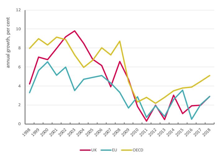
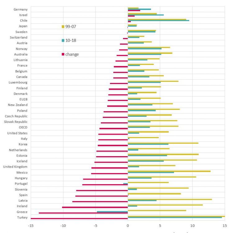
The most concrete measure of austerity is government expenditure, with the most readily available statistics for ‘general government final consumption expenditure’ (i.e. excluding investment and welfare payments). Figures 1 and 2 also introduce the graphical approach used throughout the paper: first a time series of country groupings (OECD and euro area) with the UK; and then a comparison across all OECD countries of pre- and post-crisis growth, excluding the global recession. Other points to note are that much of the analysis is done in cash terms; OECD averages are either weighted by country size (‘total’) or simple averages across countries (‘average’).[3]

Even from the start, a degree of caution was evident. At the macroeconomic level, governments generally cut back on the growth of spending. Furthermore, cuts were moderated from 2012 as the global economy abruptly weakened. Strikingly the UK Treasury relaxed austerity by even less than the EA and has continued to maintain very low spending growth (though change is underway in 2019). Overall, across the OECD, government spending growth reduced from 7.9 per cent a year in the decade before the crisis, to 2.4 per cent over 2010-2012, and has gradually increased to 5 per cent over subsequent years to 2018.

By country: Germany, Israel, Chile, Japan and Sweden stand apart with increased or (virtually) unchanged expenditure growth after the crisis. Spending growth has been cut in the vast majority of countries; however, only Portugal and Greece have endured actual cuts in the level of spending.

Figure 2: Government spending by country, average growth

While in macroeconomic terms it is important that spending growth has generally remained positive, the present episode is exceptional because of its duration. Moreover, the actual impact on public services depends on spending keeping pace not only with inflation but also population. The Office for Budget Responsibility derive a UK measure on this basis, which shows real (current) spending per capita down 15 per cent over the past nine years and forecast to rise only 5 per cent over the next five years.[1]

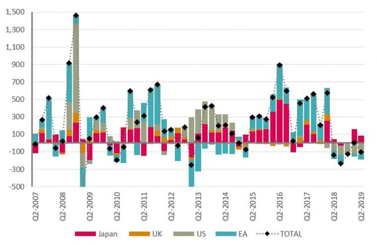
The impact of spending cuts – ‘fiscal restraint’ - has been offset by ‘monetary ease’. Central bank interest rates have been held at unprecedented low rates, and balance sheets have been expanded to a massive extent. Figure 3 below shows how quantitative easing (QE) has been shared between the major central bank (with cash amounts converted to dollars). Initially all major central banks were active. From 2013 the US and Japan took the lead. In 2015 the US stepped back, and the ECB began to take the lead. Over 2018 the US began to withdraw QE – so-called quantitative tightening (the ECB balance sheet falls because of exchange rate movements). At the time of writing, the likelihood is for resumed QE across all central banks.